Species response curves in JUICE

David Zelený & Lubomír Tichý

Institute of Botany and Zoology, Masaryk University Brno

Warning: This function in JUICE is not maintained any more. Instead, please, refere to analogical JUICE-R function for calculation of species response curves.

Determination of species response on studied gradient represents one of the basic tasks in ecology. Response curve allows estimation of species optimum and also niche width (tolerance), identifying species as generalist or specialist. Most of widely used statistical methods assume that species response on gradient have symmetrical bell shape of Gaussian curve, even if number of studies showed that this type of response occurs in real data quite rarely . Several methods dealing with problem of modeling of asymmetric species response curves were discussed in study of Oksanen & Minchin (2002a), which was together with detailed technical description in Oksanen & Minchin (2002b) taken as the base for routine built in the JUICE software and calculated in externally running R package software.

Methods for modeling response curves available in JUICE include:

1) Bell-shaped (GAUSSian) curve with traditionally symmetrical shape,

2) Generalized linear models (GLM) with polynom of 1st to 3rd degree,

3) Generalized additive models (GAM) models with optional degrees of freedom 3 to 5,

4) Huisman-Olff-Fresco models (HOF) - hierarchical set of five models with increasing complexity.

Bell-shaped curve is included mainly for reference, to show what the response shape would look like if using Gaussian model. Other three options allow quite flexible expression of different response curve shapes, each having different constrains, advantages and disadvantages. GLM models offer curves, which are completely described by equation with given number of parameters; however, the shape of its response curve is quite often somehow inappropriate or unrealistic. The GAM models are more flexible in terms of curves' shape, but their equation is non-parametric and not easily expressible. Perhaps the best option from ecological point of view is using HOF models, which are designed with stress to demands one would expect from species response curves - for example, they express only unimodal response shape, which is usually the most appropriate way when searching for species optimum on gradient (GLM and GAM with low number of degrees of polynom or freedom, respectively, can't really produce bimodal response shape, but can easily produce 'semi-bimodal' shape with inexplicit interpretation - see Fig. 3).

Available information about species is reduced only to presence-absence, even if all methods can handle also percentage or somehow transformed data. It has two reasons - first, resulting curves from presence-absence data are more 'pretty', with shapes giving more straightforward interpretation. Second, removal of information about dominance from species data makes the interpretation of resulting response curve more clear. Information about species abundance (or cover, respectively) is affected by complex factors, including competitive relations, species morphology and other biotic aspects, which all together doesn't need to be easily interpretable; on the other hand, these factors are at least partly removed, when the presence-absence transformation is used (Austin, 2002).

As any model, also response curves are just simplification of reality and their shape is strongly dependent on available dataset. One of the main assumption, which doesn't need to meet reality, is the unimodal type of species response - means that species has only one optimum along tested gradient. Even if bimodal response of species could have interesting and meaningful interpretation, it's somehow tricky in terms of determination of optimum and species tolerance, and needs to be evaluated individually for particular species. Therefore, only unimodal or monotone response of species is considered here.

Technical notes to particular modeling strategies:

1) Bell-shaped response curve is not based on the classical Gaussian equation, but on simplified equivalent polynomial model (ter Braak & Looman, 1986, Oksanen & Minchin, 2002a), which can be easily fit using generalized linear models (with logistic link function for presence-absence binomial data) and gives results close to real Gaussian curve.

2) Generalize linear models (GLM) are included in standard R package. Available models are linear, exponential and cubistic (polynom degree 1, 2 and 3, resp.), as higher polynomial degree of models would result in more then unimodal response shape. Logit link function is used; selection of model can be done manually or automatically based on AIC test criterion, selecting the model with the lowest deviance of data.

3) General additive models (GAM) are included in library 'mgcv' also available in R package. Models with fixed degree of freedom 3, 4 and 5 are available, automatic selection is also based on AIC test criterion.

4) Huisman-Olff-Fresco models (HOF) includes hierarchical set of five models: model I - flat with no response, II - monotone growing, III - monotone growing with 'plateau', IV - symmetric unimodal and V - asymmetric unimodal response. Four parameters are to be estimated - this is done using non-linear maximum likelihood estimation procedure, described in Oksanen & Minchin (2002b) and further developed by Jari Oksanen in 'gravy' package. However, 'gravy' package in some cases gives ecologically unrealistic response, and therefore we used some corrections, described in more details here ('Selfish' HOF response curves).

How species optimum and tolerance are calculated

Optimum is simply the value of gradient, where the species has the highest probability of occurrence based on particular model. If the response curve shows monotone growing, the optimum of species is identical with lowest or highest value of gradient. In case of HOF models, where flat segments of curve can occur (model I and III), optimum is localized in the middle of this flat segments (in case of model I, optimum is simply the middle-point of available gradient values).

Tolerance is determined similar to the method used in Schröder et al. (2005) - it is represented by that part of gradient, where predicted probability of species occurrence is higher than half of maximum value for predicted probability.

How to install

Calculation and drawing of response curves is processed in R software environment (R Development Core Team, 2005), which runs under complete supervision of JUICE (Tichý, 2002). Therefore, additionally to newest version of JUICE program you need to install also R package on your computer.

Install JUICE software (available for free at http://www.sci.muni.cz/botany/juice) - if you have already installed, update to the newest version (JUICE can handle species response curves up from the version 6.3.108).
Install R software package (free open source software available at http://cran.r-project.org/bin/windows/base/, install setup program).
Launch JUICE and go to File > Options > External Program Paths and setup the path to Rgui.exe file (usually placed in C:\Program Files\R\R-x.x.x\bin folder).
After importing or opening some data, go to Analysis > Species Response Curves and click on 'First run and update script' button. This will download and install all R libraries needed for calculation. You need to be connected to internet!.

Short manual

You need to import your data into JUICE, so as the short header contains the gradient data (import either from header data file or from external file via File > Import > Header data - for requested format, see JUICE manual). If you don't want to include some relevés into analysis, change their color. R program will be launched automatically by JUICE, so it doesn't need to be opened.
In JUICE menu, go to Analysis > Species Response Curves - you will launch following wizard:

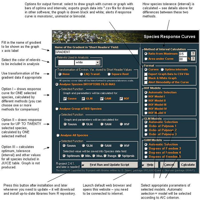
Select appropriate analysis and press Calculate button. JUICE will launch the R program and run the analysis. For large datasets, computation can last for several minutes per species (in case you calculate all species, it could take several hours). If necessary, process can be interrupted by pressing the Cancel button.
JUICE will draw the result graph and show parameters for particular curves. After finishing calculation, graph is saved also to clipboard. Results of calculation can be found at the folder C:\Program Files\R\R-x.x.x\bin\. File result_table.csv contains results of calculation (optima, interval etc.), src.bmp contains the resulting picture and graph_data.csv contains data for drawing the species curve in other sofware.

NOTE: This function is under development and suffers from several bugs - if you have any problems or questions about that, don't hasitate to send an email! (zelenysci.muni.cz, tichysci.muni.cz)

Examples of resulting graphs

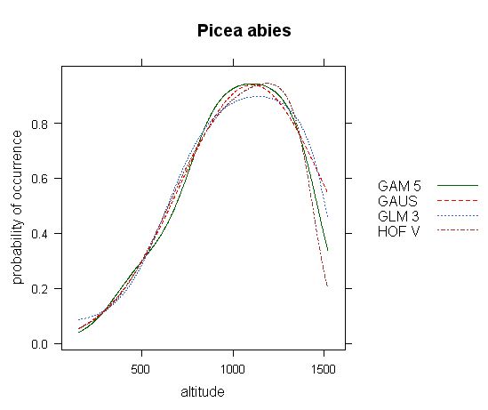
Fig.1 - Response curve of Picea abies on the gradient of altitude (based on 10.000 forest relevés data from Czech national phytosociologial database). All available models are selected, with automatic selection of model parameters.

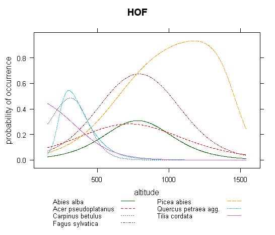
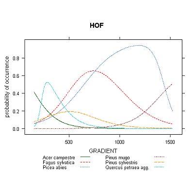
Fig.2 - Distribution of response curves of several most common tree species along altitude calculated by HOF models (the same dataset as in Fig.1).

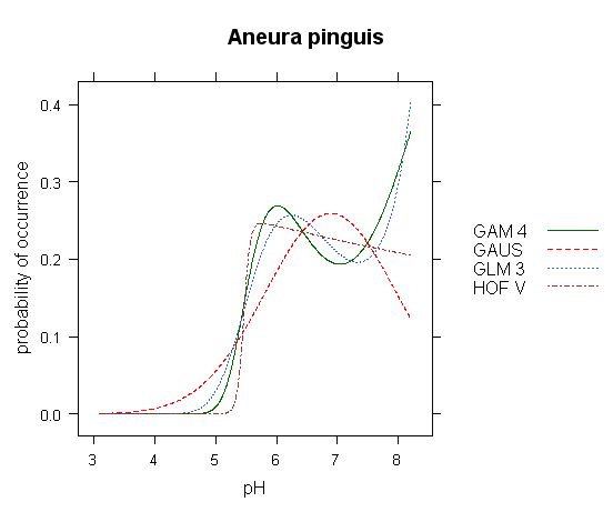
Fig.3 - Comparison of different models in response curve of Aneura pinguis along gradient of pH. Data have obvious bimodal character, reproduced by both GLM and GAM models. However, interpretetion of optimum and tolerance of these curves is somehow complicated: while GLM and GAM models put optimum to the end of gradient (pH 8.2), HOF model puts optimum into pH 5.6 and Gaussian curve somewhere inbetween - pH 6.9. Here, different models give significantly different results. (Analysis based on data of Hájek et al., ined.)

References

Austin M.P., 2002. Spatial prediction of species distribution: an interface between ecological theory and statistical modelling. Ecological Modelling 157: 101-118.

Oksanen J., Minchin P.R., 2002a. Continuum theory revisited: what shape are species responses along ecological gradients? Ecological Modelling 157: 119-129.

Oksanen J., Minchin P.R., 2002b. Non-linear maximum likelihood estimation of Beta and HOF response models. URL: http://cc.oulu.fi/~jarioksa/softhelp/hof3.pdf

R Development Core Team (2005). R: A language and environment for statistical computing. R Foundation for Statistical Computing, Vienna, Austria. ISBN 3-900051-07-0, URL http://www.R-project.org.

Schröder, H. K., Andersen H. E., Kiehl K., 2005. Rejecting the mean: Estimating the response of fen plant species to environmental factors by non-linear quantile regression. Journal of Vegetation Science 16: 373-382.

ter Braak, C.J.F, Looman, C.W.N., 1986. Weighted averaging, logistic regression and the Gaussian response model. Vegetatio 65: 3-11.

Tichý, L., 2002. JUICE, software for vegetation classification. Journal of Vegetation Science 13: 451-453.